
双重流动性之殇 —— KyberSwap 巨额被黑分析


作者: 九九 & Kong & Lisa;来源:慢雾科技
背景
据慢雾安全团队情报,2023 年 11 月 23 日,去中心化交易平台 KyberSwap 遭到攻击,攻击者获利约 5470 万美元。慢雾安全团队第一时间介入分析,并将结果分享如下:
根本原因
由于 KyberSwap Elastic 的 Reinvestment Curve(再投资曲线特性),在基础流动性与再投资流动性作为实际流动性参与计算的情况下,使得池子通过 calcReachAmount 函数在刻度边界计算兑换所需的代币数量大于预期,造成下一价格 sqrtP 超过边界刻度的 sqrtP,且池子使用不等号对 sqrtP 进行检查,导致协议未按预期的通过 _updateLiquidityAndCrossTick 更新流动性。
前置知识
在分析开始前,我们需要了解关于 KyberSwap 一些关键性知识以便理解本次分析内容。
KyberSwap 是一个链上去中心化交易平台,其具有一种新型的流动性优化模型——KyberSwap Elastic。该模型采用的集中流动性做市商机制使 LP 能够将流动性分配给定制的价格区间,并且引入再投资曲线,自动为 LP 复利在池子中闲置的流动性费用。
首先,何谓集中流动性做市商(CLMM)?与 Uniswap v3 类似,流动性提供者可以将其资金在自定义价格区间内提供流动性,只有当价格落在此区间内,其流动性才会被使用。Uniswap v3 (https://blog.uniswap.org/uniswap-v3) 与 KyberSwap (https://docs.kyberswap.com/liquidity-solutions/kyberswap-elastic) 都提供了详细的文档进行解释说明,我们这里以一个简易的 ETH/USDC 池子图例来说明阅读此文章所需了解的知识:
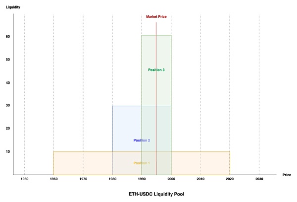
From: KyberSwap Elastic Liquidity Concept (https://docs.kyberswap.com/liquidity-solutions/kyberswap-elastic/concepts/concentrated-liquidity#liquidity-tracking-lp-contributions-at-a-specific-price)
以上是具有三个相同流动性仓位组成的 ETH/USDC 池子,当前价格为 1995。在 CLMM 中,价格范围被成为 tick-range。仓位 1 流动性所在的 tick 范围为 1960-2020,仓位 2 流动性所在的 tick 范围为 1980-2000,仓位 3 流动性所在的 tick 范围为 1990-2000。
由图可得当前范围所在位置是流动性最好的范围,三个仓位流动性在 tick 1990-2000 上重合。当 ETH 价格下跌至 1985 时,其价格将向左移动越过 tick 1990 的范围,此时其将要离开仓位 3 的流动性范围,但仍在仓位 1 和 2 的流动性范围中,因此将会更新新范围内的流动性,将仓位 3 的流动性排除。而当 ETH 价格上涨至 2005 时,其价格将向右移动越过 tick 2000 的范围,此时将排除仓位 2 和 3 的流动性,但其仍在仓位 1 范围里。即当价格跨过流动性边界时必将更新流动性,或增加或减少。
与 Uniswap v3 不同的是,KyberSwap Elastic 创新的引入了一个新特性 —— Reinvestment Curve(再投资曲线)。这是一个额外的 AMM 池,其将用户在池子中兑换收取的费用累积到其中,其曲线支持从 0 到无穷的价格范围。KyberSwap Elastic 通过过将再投资曲线与原始价格曲线进行聚合(即曲线分离,但资金仍在同一个池中),使得 LP 的费用及时在价格超出其仓位范围时也能复利赚取收益。
简单了解 KyberSwap Elastic 的机制后,我们对攻击步骤进行分析。
攻击步骤分析
此处以攻击交易 0x485...0f3 为例进行分析:
1. 攻击者首先从 AAVE 中闪电贷出 2000 枚 WETH,并在 KyberSwap 的池子中用 6.8496 枚 WETH 兑换成 frxETH,使 frxETH 的价格越过流动性提供者的所有仓位范围。此时当前的价格数值 sqrtP(当前价格乘以 2^96 的平方根表示)被拉升至 20282409603651670423947251286016,位于 tick 110909 上。
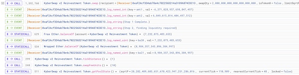
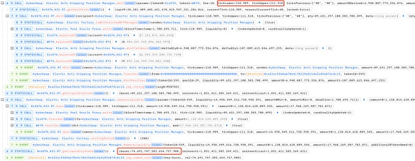
2. 接下来攻击者在指定的价格区间 [110909,111310] 添加了 0.006948 枚 frxETH 和 0.1078 枚 WETH 作为流动性,随后又移除了部分的流动性,最终将该价格区间里的流动性数值控制在 74692747583654757908 以使得流动性符合后续攻击计算时所需的数额。此时 tick [110909,111310] 区间只有攻击者一人拥有流动性,tick 111310 的价格数值 sqrtP 为 20693058119558072255662180724088。
3. 之后攻击者在当前价格刻度 110909 用 387.17 枚 WETH 兑换出 0.005789 枚 frxETH。此次大额兑换将当前价格数值 sqrtP 拉升至 20693058119558072255665971001964,超过了边界刻度 111310 上的 sqrtP。
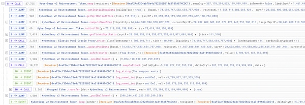
4. 最后攻击者从略大于价格刻度 111310 的 sqrtP 处,使用 0.005868 枚 frxETH 反向兑换出 396.2 枚 WETH,兑换后价格落回 [110909,111310] 刻度范围内。此时攻击者已经获利,其反向兑换比正向兑换多换出了约 9 枚 WETH。
为何如此朴实无华的攻击步骤却能换出多于预期的资金呢?这与 KyberSwap Elastic 的再投资曲线有着极大的关联,我们接下来通过详细剖析来揭秘其获利方式。
攻击原理剖析
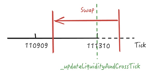
通过上述步骤我们知道在进行最后一步反向兑换时换出了多于预期的资金,在进行兑换时当前 sqrtP 为 20693058119558072255665971001964,这大于攻击者添加流动性时的 tickUpper 111310 所在的价格,我们用刻度图示意其所在的位置。
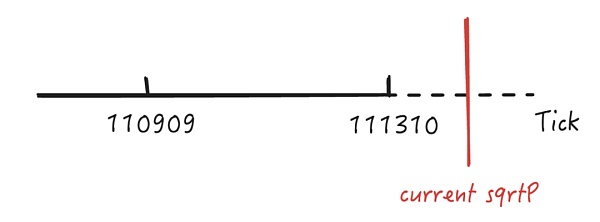
由于超过了攻击者添加的流动性刻度 [110909,111310] 范围,因此当前 sqrtP 所在的位置理论上是没有流动性的,其在兑换过程中只能向左跨过 111310 刻度才能获得有效的流动性进行兑换,我们跟进查看其是否如预期进行兑换。
如下图所示,当我们查看当前 sqrtP 所在刻度的流动性时,我们发现不考虑重投资曲线的情况下,这里本该是 0 流动性的范围内却非预期的出现了大量流动性且远大于重投资曲线的流动性,并且流动性数额与刻度 [110909,111310] 范围内一致。
这使得在进行兑换时,将在刻度 111310 进行有效的代币兑换,如下图所示。
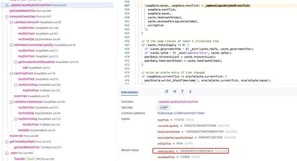
在刻度 111310 进行有效兑换后,sqrtP 将跨过此刻度进入 [110909,111310] 范围兑换剩余的代币。回顾前置知识我们知道在跨越流动性仓位范围时将进行流动性更新,在 KyberSwap Elastic Pool 中会通过 _updateLiquidityAndCrossTick 函数将 [110909,111310] 范围内的流动性加入曲线中以参与代币兑换,如下图所示。
这将使得刻度 [110909,111310] 范围内的有效流动性会与刻度 111310 右边多出的虚假流动性相加,导致在刻度 [110909,111310] 范围内进行兑换时的总有效流动性远大于预期,如下图所示,有效流动性比预期增加了一倍。
而由于当前刻度范围内流动性的增加,使得池子的深度比预期更好,因此攻击者可以获得比预期多的资金,这些额外的资金来自于池子中其他刻度范围的流动性。
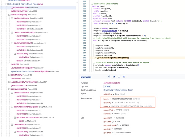
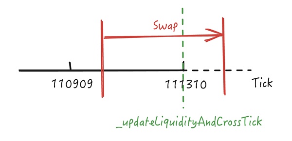
而为什么在刻度 111310 右边会多出非预期的流动性,且流动性数量还与 [110909,111310] 范围的流动性相同呢?唯一的解释只能是在前一次兑换过程中池子并未按照预期进行流动性更新操作。如下图所示,理论上在进行前一次兑换跨过 tick 111310 时,也应该调用 _updateLiquidityAndCrossTick 函数,更新 sqrtP 进入 tick 111310 右边后的流动性。
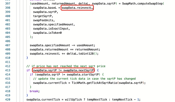
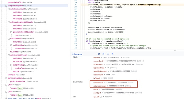
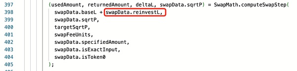
我们实际分析此兑换过程,在进行兑换时 Pool 将通过 computeSwapStep 函数计算用于兑换的实际数额,以及兑换费用和新的 sqrtP 价格数值。理论上,在跨越流动性范围时,计算的 sqrtP 结果将会是落在范围边界的刻度 111310 的 sqrtP。但实际上新的 sqrtP 已经超过了刻度 111310 的 sqrtP。如下图所示,刻度 111310 的 sqrtP 为 20693058119558072255662180724088,但实际 sqrtP 却是 20693058119558072255665971001964。
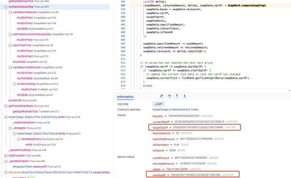
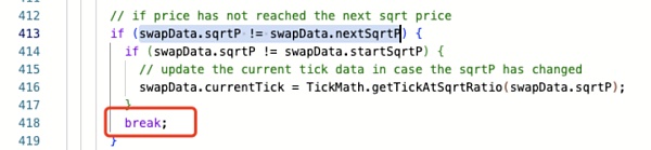
由于新的 sqrtP 并未落在边界刻度 111310 的 sqrtP 上,即 swapData.sqrtP != swapData.nextSqrtP,这将使得池子认为当前 sqrtP 还在 [110909,111310] 范围内,因此将跳出流动性检查操作,不会触发 _updateLiquidityAndCrossTick 函数进行流动性更新!
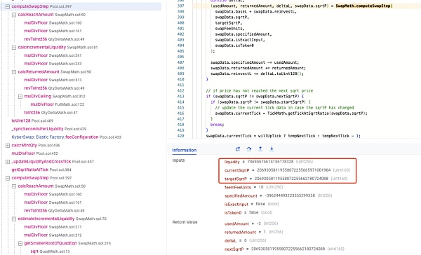
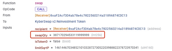
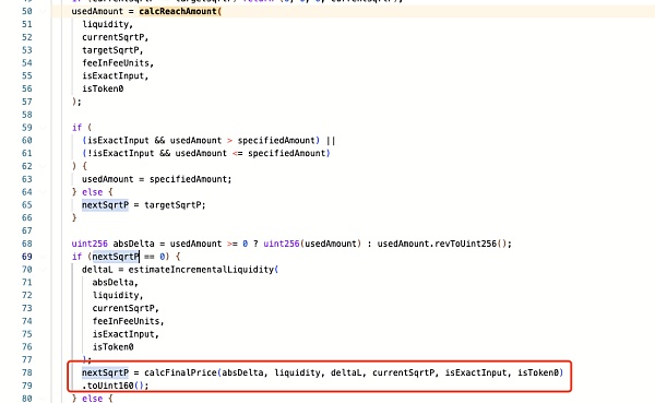
但为什么会出现新的 nextSqrtP 未落在边界上的情况呢?通过分析 calcReachAmount 计算,我们可以发现攻击兑换的数额 387170294533119999999 正好小于当前范围内的流动性数量 387170294533120000000。
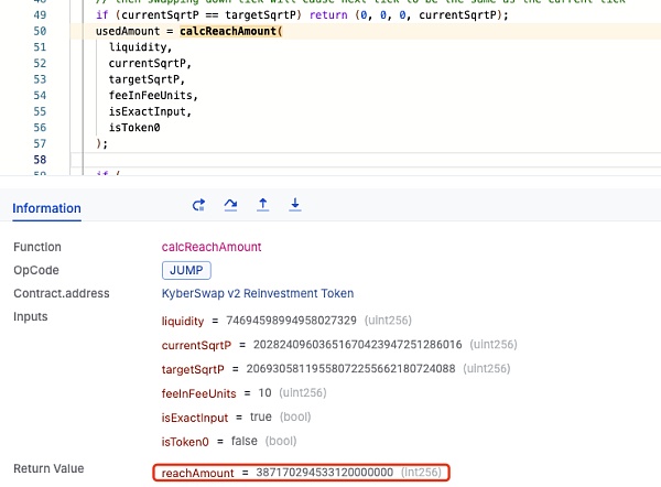
这使得 nextSqrtP 不会被赋值为 targetSqrtP,而是仍然为 0,因此其将直接通过 calcFinalPrice 函数进行最后的 sqrtP 计算,这使得其计算结果大于刻度 111310 的 sqrtP。
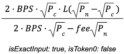
因此 calcReachAmount 函数是关键,其用于计算从 currentSqrtP 到达 targetSqrtP 的兑换中所需的代币数量。通过分析其计算公式,我们可以知道其计算结果主要取决于当前流动性 L,而当前流动性 L 是基础流动性和再投资流动性的总和。
我们都知道在 Uniswap v3 中并没有再投资曲线的特性,因此是否是因为加入了再投资流动性导致 calcReachAmount 的计算结果比预期的大呢?
通过测试,在不包含再投资流动性的情况下,calcReachAmount 计算结果为 387160697969657129472,这小于攻击所兑换的数量 swapQty 387170294533119999999。
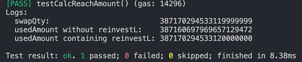
而在不包含再投资流动性的情况下 computeSwapStep 计算的 sqrtP 则刚好落在刻度 111310 上:
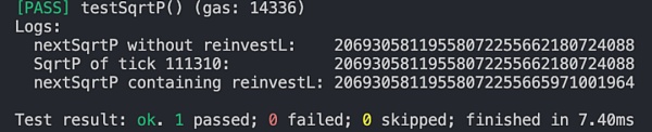
因此真相水落石出,由于 KyberSwap Elastic 的 Reinvestment Curve(再投资曲线)特性,在使用基础流动性与再投资流动性计算从当前 sqrtP 到刻度边界 sqrtP 的兑换中,所需的代币数量将大于预期,这导致了兑换后的 sqrtP 超过刻度边界的 sqrtP,使得协议认为当前刻度范围内的流动性已经满足了兑换所需,进而停止对越过边界刻度进行流动性更新的操作。
MistTrack 分析
KyberSwap Exploiter 1:0x50275e0b7261559ce1644014d4b78d4aa63be836
KyberSwap Exploiter 2:0xc9b826bad20872eb29f9b1d8af4befe8460b50c6
KyberSwap Exploiter 3:0xae7e16cAa7a4d572FfF09924Bf077a89485850Cb
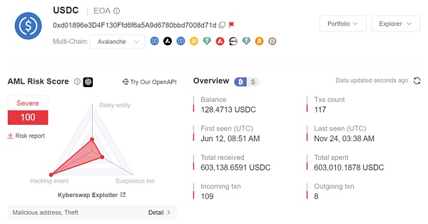
KyberSwap Exploiter 4:0xd01896e3D4F130Ffd6f6a5A9d6780bbd7008d71d
据 MistTrack 分析,KyberSwap 攻击者共获利超 5470 万美元,涉及 Ethereum、BSC、Arbitrum、Optimism、Polygon、BASE、Scroll、Avalanche 链。
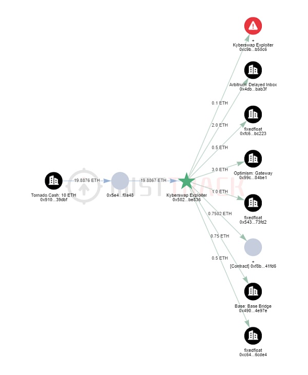
在 Ethereum 上,KyberSwap Exploiter 1 的初始资金来自 Tornado Cash 转入的 20 ETH。其中 0.1 ETH 被转移到 KyberSwap Exploiter 2,2 ETH 被转移到 FixedFloat,6.5 ETH 被分别跨链到 Arbitrum, Optimism, Scroll, Base 链。而 KyberSwap Exploiter 2 则获利价值超 758 万美元的 Token,包含 USDC, WETH, KNC 等,暂未转移。
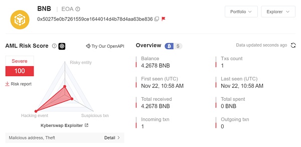
在 BSC 上,KyberSwap Exploiter 1 收到了 FixedFloat 转入的 4.2678 BNB,作为余额暂未转移。
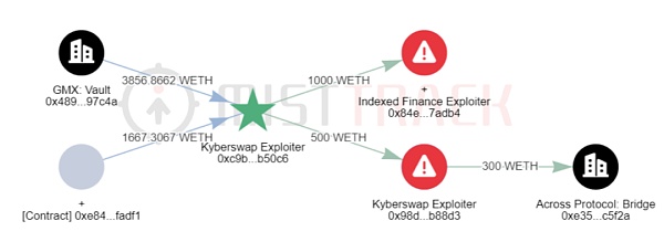
在 Arbitrum 上,KyberSwap Exploiter 2 获利价值超 2029 万美元的 Token,包含 WBTC, WETH, ARB, DAI 等,其中 500 WETH 转移到 0x98d69d3ea5f7e03098400a5bedfbe49f2b0b88d3,该地址将 300 WETH 跨链到以太坊,暂未转移。值得注意的是,KyberSwap Exploiter 2 将 1,000 WETH 转移到 Indexed Finance Exploiter 的地址 0x84e66f86c28502c0fc8613e1d9cbbed806f7adb4。
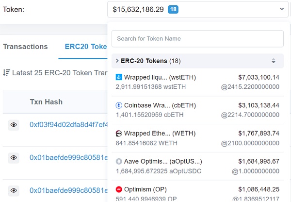
在 Optimism 上,KyberSwap Exploiter 2 获利超 1564 万美元的 Token,包含 wstETH, WETH, OP, DAI 等,暂未转移。
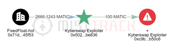
在 Polygon 上,KyberSwap Exploiter 1 的初始资金来自 FixedFloat 转入的 2,666.1243 MATIC,接着将 100 MATIC 转到 KyberSwap Exploiter 2,目前 Exploiter 1 余额为 2,564.0016 MATIC;而 KyberSwap Exploiter 2 获利超 293 万美元的 Token,包含 WBTC, WETH, DAI 等,暂未转移;KyberSwap Exploiter 3 获利超 575 万美元的 Token,包含 wstETH, USDT, USDC 等,并将大部分 Token 转移到地址 0xa4c92d7482066878bb1e2c0510f42b20d79a7ea9。
在 BASE 上,KyberSwap Exploiter 2 获利超 195 万美元的 Token,包含 USDC, WETH 等,暂未转移。
在 Avalanche 上,KyberSwap Exploiter 1 的初始资金来自 FixedFloat 转入的 49 AVAX;而 KyberSwap Exploiter 2 获利超 2.35 万美元的 Token,包含 293.0756 WAVAX, 17,316.0305 USDC,暂未转移;KyberSwap Exploiter 4 获利超 56.5 万美元的 Token,包含 WAVAX, USDC 等,并将 USDC 转移到地址 0x9296fa3246f478e32b05d4dde35176d927be703f。
慢雾安全团队已拉黑相关地址,大部分资金仍未转移,我们将持续监控资金异动。
结论
此次攻击事件的根本原因在于计算当前价格到边界刻度价格的兑换中,所需的代币数量会因为 KyberSwap Elastic 的再投资曲线而将流动性多加上手续费复利的部分,从而造成其计算结果比预期大,可以覆盖用户兑换所需,但实际价格已经越过了边界刻度,使得协议认为当前刻度范围内的流动性已经满足了兑换所需,故而未进行流动性更新。最终导致反向兑换跨过边界刻度时流动性增加了两次,使得攻击者获得了多于预期的代币。
慢雾安全团队建议在设计经济模型时,应对边界条件进行充分测试,并且严格判断流动性与价格而不是使用不等号进行检查。
参考
攻击者地址:0x50275e0b7261559ce1644014d4b78d4aa63be836
攻击合约:0xaf2acf3d4ab78e4c702256d214a3189a874cdc13
相关攻击交易:
0x485e08dc2b6a4b3aeadcb89c3d18a37666dc7d9424961a2091d6b3696792f0f3
0x09a3a12d58b0bb80e33e3fb8e282728551dc430c65d1e520fe0009ec519d75e8
0x396a83df7361519416a6dc960d394e689dd0f158095cbc6a6c387640716f5475
According to the information of the slow fog security team, the decentralized trading platform was attacked, and the attacker made a profit of about 10,000 US dollars. The slow fog security team immediately intervened in the analysis and shared the results as follows. The fundamental reason is that the reinvestment curve characteristics of the pool make the number of tokens required for redemption at the scale boundary calculated by the function larger than expected, resulting in the next price exceeding the boundary scale, and The pool uses unequal pairs to check, which leads to the agreement failing to update the liquidity pre-knowledge as expected. Before the analysis begins, we need to know some key knowledge in order to understand that the content of this analysis is a centralized trading platform with a new liquidity optimization model. The centralized liquidity market maker mechanism adopted in this model enables the liquidity to be allocated to a customized price range and the reinvestment curve to automatically be the first liquidity expense with compound interest idle in the pool. First of all, what is centralized liquidity? Market makers and similar liquidity providers can provide their funds with liquidity within a self-defined price range. Only when the price falls within this range will their liquidity be used, and detailed documents have been provided to explain it. Here, we use a simple pool legend to illustrate the knowledge needed to read this article. The above is a pool composed of three positions with the same liquidity. The current price range is in the middle, and the range where the liquidity is called the position is the position. The range of liquidity is the range of position liquidity. It can be seen from the figure that the current range is the best range of liquidity. The liquidity of three positions overlap on the top. When the price falls to, its price will move to the left. At this time, it will leave the liquidity range of the position, but it is still in the liquidity range of the position sum. Therefore, it will update the liquidity in the new range to exclude the liquidity of the position, and when the price rises to, its price will move to the right. At this time, the position will be excluded. But it is still in the range of positions, that is, when the price crosses the liquidity boundary, it will update the liquidity or increase or decrease. The difference is that it innovatively introduces a new characteristic reinvestment curve, which is an additional pool, and its curve supports the price range from infinite to infinite. By aggregating the reinvestment curve with the original price curve, that is, the curve is separated, but the funds are still in the same pool, so that the expenses exceed their positions in time. After a simple understanding of the mechanism, we will analyze the attack steps. Here, we will analyze the attack transaction as an example. The attacker first lent RMB from it and exchanged RMB in the pool to make the price cross all the positions of the liquidity provider. At this time, the square root of the current price multiplied by the current price indicates that it has been pulled up to the top. Next, the attacker added RMB and RMB as liquidity in the specified price range, and then removed it. Part of the liquidity finally controls the liquidity value in the price range to make the liquidity meet the amount required for subsequent attack calculation. At this time, only the attacker has the liquidity price value, and then the attacker exchanges gold for gold on the current price scale. This large exchange has raised the current price value to beyond the boundary scale, and the last attacker uses gold from a place slightly larger than the price scale. After the exchange, the price falls back into the scale range. At this time, the attacker has After making a profit, the reverse exchange has exchanged more than the forward exchange. Why can such an unpretentious attack step exchange more funds than expected? This has a great correlation with the reinvestment curve. We will reveal its profit mode through detailed analysis. Through the above steps, we know that the last step of reverse exchange has exchanged more funds than expected. At present, it is greater than the price at which the attacker added liquidity. We use the scale chart to indicate. Its location is beyond the liquidity scale added by the attacker, so its current location is theoretically illiquid. It can only cross the scale to the left in the exchange process to obtain effective liquidity for exchange. We follow up to see if it is exchanged as expected, as shown in the following figure. When we look at the liquidity of the current scale, we find that there is a lot of liquidity unexpectedly in the scope of liquidity without considering the reinvestment curve. Much greater than the liquidity of the reinvestment curve, and the amount of liquidity is consistent with the scale range, which makes the effective exchange of tokens at the scale as shown in the figure below. After the effective exchange at the scale, the remaining tokens will be exchanged across the scale. We know that the liquidity will be updated when crossing the liquidity position range, and the liquidity within the range will be added to the curve through functions to participate in the exchange of tokens as shown in the figure below, which will make it within the scale range. The effective liquidity of the pool will be added to the false liquidity on the right side of the scale, resulting in the total effective liquidity in the scale range being much greater than expected. As shown in the following figure, the effective liquidity has doubled than expected, and the depth of the pool is better than expected due to the increase of liquidity in the current scale range, so the attacker can get more funds than expected. These extra funds come from the liquidity of other scales in the pool. Why is there more unexpected liquidity on the right side of the scale? And the amount of liquidity is the same as the liquidity of the range. The only explanation can only be that the pool did not carry out the liquidity update operation as expected in the previous exchange process, as shown in the following figure. Theoretically, the function should also be called to update the liquidity after entering the right during the previous exchange crossing. We actually analyze this exchange process, and the actual amount used for exchange, the exchange fee and the new price value will be calculated by the function when crossing the liquidity range. It will fall on the scale of the range boundary, but in fact the new one has exceeded the scale as shown in the following figure, but it is actually because the new one has not fallen on the scale of the boundary, that is, it will make the pool think that it is still in the range at present, so it will jump out of the liquidity check operation and will not trigger the function to update the liquidity, but why is there a new situation that does not fall on the boundary? Through analysis and calculation, we can find that the amount of attack exchange is just less than the amount of liquidity in the current range, which makes it not be assigned as but still as, so it will make the final calculation directly through the function, which makes its calculation result 比特币今日价格行情网_okx交易所app_永续合约_比特币怎么买卖交易_虚拟币交易所平台
注册有任何问题请添加 微信:MVIP619 拉你进入群

打开微信扫一扫
添加客服
进入交流群
1.本站遵循行业规范,任何转载的稿件都会明确标注作者和来源;2.本站的原创文章,请转载时务必注明文章作者和来源,不尊重原创的行为我们将追究责任;3.作者投稿可能会经我们编辑修改或补充。